Factor Models

Basics

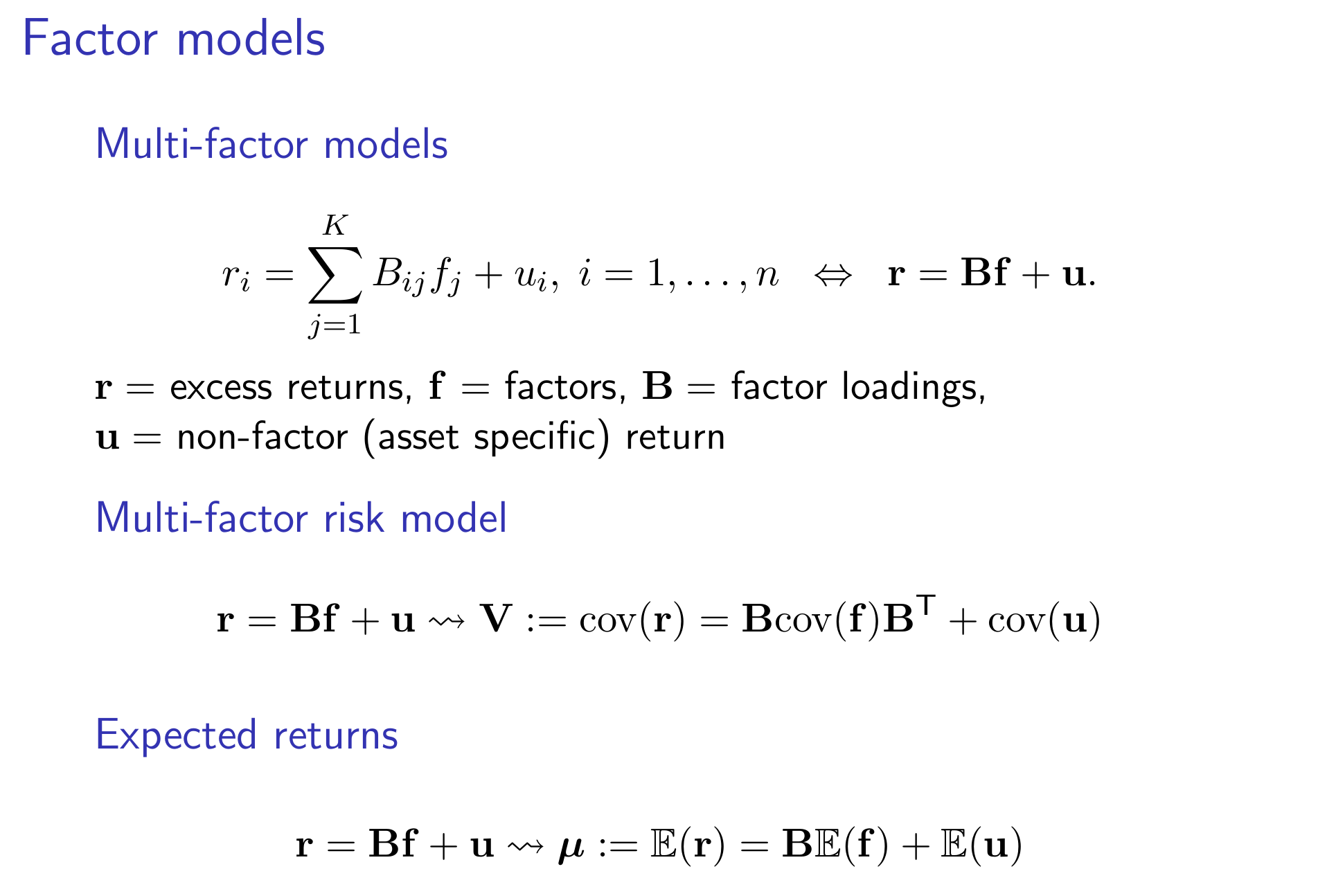
The following two slides are very good summary of the basic forms and we do not need to repeat. But do notice that for \(n\) risky assets and \(k\) factors, we have \(\mathbf{B}\in \mathbb{R}^{n \times k}\).

As we can notice, though the meaning of loadings and factors can be defined, they are hard to calculate. You could assume you have one of them, and then regress to get the other one. That's why there are many variations of the factor models, because they start from different assumptions.

Estimation of Factor Models - Assume Observable Loadings

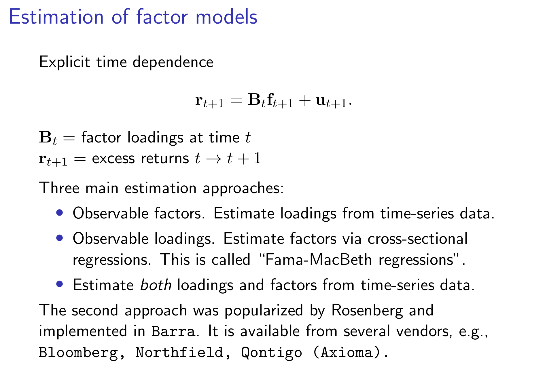
We interpret \(\mathbf{r}\) as the factor returns, and assume that loadings are observable and change with time \(t\), then, this is called a Fama-Macbeth Regression in the following form:

\[ \min _{\mathbf{f}_{t+1}}\left\|\mathbf{r}_{t+1}-\mathbf{B}_t \mathbf{f}_{t+1}\right\|^2 \rightsquigarrow \mathbf{f}_{t+1}=\left(\mathbf{B}_t^{\top} \mathbf{B}_t\right)^{-1} \mathbf{B}_t^{\top} \mathbf{r}_{t+1} \]

If we do have weights to assign for each observation, we can do weighted least square

\[ \left\|\mathbf{r}_{t+1}-\mathbf{B}_t \mathbf{f}_{t+1}\right\|_{\mathbf{D}^{-1}}^2=\left(\mathbf{r}_{t+1}-\mathbf{B}_t \mathbf{f}_{t+1}\right) \mathbf{D}^{-1}\left(\mathbf{r}_{t+1}-\mathbf{B}_t \mathbf{f}_{t+1}\right) \]

where \(\mathbf{D}\) is diagonal whose entries estimate the asset-specific variances. Popular choice: \(\mathbf{D}^{-1}=\) diagonal matrix of square roots of market capitalizations.

Finally, use \(\mathbf{f}_{t+1}\) and \(\mathbf{u}_{t+1}:=\mathbf{r}_{t+1}-\mathbf{B}_t \mathbf{f}_{t+1}, t=0,1, \ldots, T-1\) to estimate \(\operatorname{cov}(\mathbf{f})\) and \(\operatorname{cov}(\mathbf{u})\).

Translate historical into predicted. The historical data helps to estimate factors and idiosyncratic risks. Take expectation of them to get \(\boldsymbol{\mu}=\mathbb{E}(r)\) and \(\operatorname{cov}(r)\) to form portfolios.

Alpha

Now we have fit the factor model, and the APT theory states that the expected returns of risky assets should be well explained by the factors (all premia is compensation for exposure to certain risk factors). In this case, if \(\mathbf{f}\) is complete, then we should see \(\mathbb{E}(\mathbf{u})=0\).

CAPM is one of the pricing models which assumes the following form,

\[ \mathbf{r}=\boldsymbol{\beta} r_M+\mathbf{u} \rightsquigarrow \boldsymbol{\mu}=\boldsymbol{\beta} \mu_M+\mathbb{E}(\mathbf{u}) \]

If it really holds, then \(\boldsymbol{\alpha}:=\mathbb{E}(\mathbf{u})=\mathbf{0}\). We could test it in a regression model to see if there is any statistically significant intercept term.