Dynamic Programming
Problem Setup

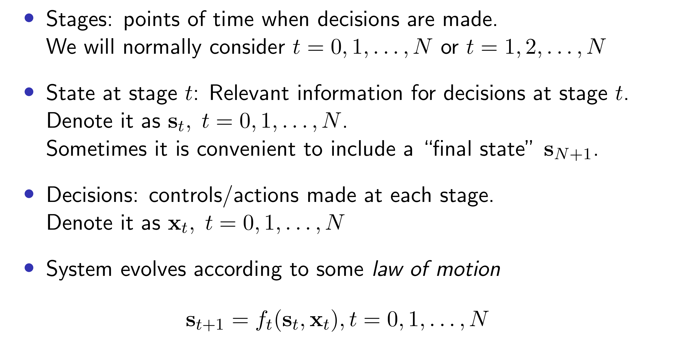
Our goal is to decide a series of actions \(\mathbf{x}_t, t=0,1, \ldots, N\) to maximize or minimize the total cost / reward. In this case, we have intermediate rewards \(g_t\left(\mathbf{s}_t, \mathbf{x}_t\right)\).
\[
\sum_{t=0}^N g_t\left(\mathbf{s}_t, \mathbf{x}_t\right)+g_{N+1}\left(\mathbf{s}_{N+1}\right)
\]
Suppose we are maximizing reward:
\[
J\left(\mathbf{s}_0\right):=\max _{\mathbf{x}_0, \ldots, \mathbf{x}_T}\left[\sum_{t=0}^T g_t\left(\mathbf{s}_t, \mathbf{x}_t\right)+g_{T+1}\left(\mathbf{s}_{T+1}\right)\right] .
\]
Consider the value-to-go of the tail problem starting at stage \(t\) :
\[
J_t\left(\mathbf{s}_t\right):=\max _{\mathbf{x}_t, \ldots, \mathbf{x}_T}\left[\sum_{\tau=t}^T g_\tau\left(\mathbf{s}_\tau, \mathbf{x}_\tau\right)+g_{T+1}\left(\mathbf{s}_{T+1}\right)\right]
\]
The Bellman's optimality principle is,
\[
\begin{aligned}
J_t\left(\mathbf{s}_t\right) & =\max _{\mathbf{x}_t}\left[g_t\left(\mathbf{s}_t, \mathbf{x}_t\right)+J_{t+1}\left(\mathbf{s}_{t+1}\right)\right] \\
& =\max _{\mathbf{x}_t}\left[g_t\left(\mathbf{s}_t, \mathbf{x}_t\right)+J_{t+1}\left(f_t\left(\mathbf{s}_t, \mathbf{x}_t\right)\right)\right] .
\end{aligned}
\]
Notice that in the second step, we have plugged in the law of motion. At each stage, we are maximizing the current reward plus the deferred / value to go in the next stage.
Similarly, in a stochastic case, we can maximize the expectation here,
\[
\begin{aligned}
& J_t\left(\mathbf{s}_t\right)=\max _{\mathbf{\mathbf { x } _ { t }}} \mathbb{E}_t\left[g_t\left(\mathbf{s}_t, \mathbf{x}_t, \boldsymbol{\omega}_t\right)+J_{t+1}\left(\mathbf{s}_{t+1}\right)\right] \\
& =\max _{\mathbf{x}_t} \mathbb{E}_t\left[g_t\left(\mathbf{s}_t, \mathbf{x}_t, \boldsymbol{\omega}_t\right)+J_{t+1}\left(f_t\left(\mathbf{s}_t, \mathbf{x}_t, \boldsymbol{\omega}_t\right)\right)\right] \\
&
\end{aligned}
\]
Dynamic Portfolio Optimization (simple case when myopic is optimal)
Suppose we start from \(W_0\) invest in multiple periods, aiming to maximize the utility of the terminal wealth \(\mathbb{E}\left(U\left(W_N\right)\right)\), how should we decide the holdings at each period.
\[
W_N=W_0 \cdot \prod_{t=0}^{N-1}\left(R_{f, t+1}+\mathbf r_{t+1}^{\top} \mathbf x_t\right)
\]
We see multiplications over periods. Specifically, if the returns over time periods are independent, and we use a power utility function \(U(w)=\frac{w^{1-\gamma}}{1-\gamma}\), then a myopic strategy is optimal. We only need to maximize the utility for the next period only, and repeat.
\[
\mathbb{E}\left(W_N^{1-\gamma}\right)=W_0^{1-\gamma} \cdot \mathbb{E}\left(\prod_{t=0}^{N-1} R_{p, t+1}^{1-\gamma}\right)\\
\mathbb{E}\left(W_N^{1-\gamma}\right)=W_0^{1-\gamma} \cdot \prod_{t=0}^{N-1} \mathbb{E}\left(R_{p, t+1}^{1-\gamma}\right)\\
\max _{\mathbf{x}_0, \ldots, \mathbf{x}_{N-1}} \mathbb{E}\left(U\left(W_N\right)\right) \Leftrightarrow \prod_{t=0}^{N-1} \max _{\mathbf{x}_t} \mathbb{E}\left(U\left(R_{p, t+1}\right)\right)
\]
If we instead have \(U(w)=\log (w)\), which further simplifies the problem, even when returns are not independent, since we just need to sum the log returns. Our goal just becomes maximizing the log returns in each single period. So a myopic strategy is optimal.
