Support Vector Machines
Table of Contents
Support Vector Classifier
The idea of SVM comes from solving the binary classification problem by separating the $p$ dimensional space using a $p-1$ dimensional hyperplane. If $p=2$, then the “hyperplane” will just be a line.
To make the boundary of classes less vulnerable to slight change of “support vectors” (which are observations close to the hyperplane that have direct impact on the hyperplane), we introduce the support vector classifier that allow some misclassifications (soft margin classifier). They will offer,
- greater robustness of individual observations
- better classifications for most training observations
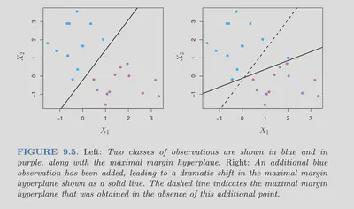
The chart below shows that a maximal margin hyperplane always try to classify all the observations on the right side, and then maximize the margin. So it can be very volatile.

SVC introduces a parameter $C$ which allows some tolerance to violate the margin. The goal remains to be maximizing the margin with this new constraint. The formal problem step up is as follows
$$ \begin{aligned} &\underset{\beta_{0}, \beta_{1}, \ldots, \beta_{p}, \epsilon_{1}, \ldots, \epsilon_{n}, M}{\operatorname{maximize}} M\\ &\text { subject to } \sum_{j=1}^{p} \beta_{j}^{2}=1 \text {, }\\ &y_{i}\left(\beta_{0}+\beta_{1} x_{i 1}+\beta_{2} x_{i 2}+\cdots+\beta_{p} x_{i p}\right) \geq M\left(1-\epsilon_{i}\right) \text {, }\\ &\epsilon_{i} \geq 0, \quad \sum_{i=1}^{n} \epsilon_{i} \leq C, \end{aligned} $$When we classify a new observation, say $x^{\star}$, we look at the sign of $f\left(x^{\star}\right)=\beta_{0}+\beta_{1} x_{1}^{\star}+\cdots+\beta_{p} x_{p}^{\star}$, as only the side of the hyperplane is decisive in classifying.
Support Vector Machine
The solution of the above SVC problem, happens to include only the inner products of the observations. In other words, denote $r$ dimensional vectors $a$ and $b$, and the inner product is $\langle a, b\rangle=\sum_{i=1}^{r} a_{i} b_{i}$. Since SVC is only determined by the support vectors, therefore, only the collection $\mathcal{S}$ of these support points are needed. The solution can be written as:
$$ f(x)=\beta_{0}+\sum_{i \in \mathcal{S}} \alpha_{i}\left\langle x, x_{i}\right\rangle $$If we change this inner product to other forms, to enlarge the feature space and accommodate a non linear boundary, then the solution of SVC can be written as
$$ f(x)=\beta_{0}+\sum_{i \in \mathcal{S}} \alpha_{i} K\left(x, x_{i}\right) $$Some important kernels,
Polynomial kernel of dimension $d$ : $K\left(x_{i}, x_{i^{\prime}}\right)=\left(1+\sum_{j=1}^{p} x_{i j} x_{i^{\prime} j}\right)^{d}$
Radial Kernel: $K\left(x_{i}, x_{i^{\prime}}\right)=\exp \left(-\gamma \sum_{j=1}^{p}\left(x_{i j}-x_{i^{\prime} j}\right)^{2}\right)$
The kernel measures the similarity between points, so higher $\gamma$ above will push the kernel values smaller, which leads to more local behavior. Only nearby training observations have an effect on the class label of a test observation. If $x$ is far away from the $x_i$, then $x_i$ has little impact of $f(x)$.
Connection with Logistic
A typical way to construct the objective function is
$$ \operatorname{minimize}_{\beta_{0}, \beta_{1}, \ldots, \beta_{p}}\{L(\mathbf{X}, \mathbf{y}, \beta)+\lambda P(\beta)\} $$Regardless of the $P(\beta)$ for now, as they are similar between methods, and focus on the loss,
For logistic regression, the loss term is,
$$ L(\mathbf{X}, \mathbf{y}, \beta)=\sum_{i=1}^{n}\left(y_{i}-\beta_{0}-\sum_{j=1}^{p} x_{i j} \beta_{j}\right)^{2} $$For SVM, on the other hand, minimize the hinge loss,
$$ L(\mathbf{X}, \mathbf{y}, \beta)=\sum_{i=1}^{n} \max \left[0,1-y_{i}\left(\beta_{0}+\beta_{1} x_{i 1}+\cdots+\beta_{p} x_{i p}\right)\right] $$Why the hinge loss makes sense? Since the classifier is solely dependent on the support vectors, all the points that are correctly put on the sides of the margin will have $y_{i}\left(\beta_{0}+\beta_{1} x_{i 1}+\cdots+\beta_{p} x_{i p}\right) \geq 1$, which contributes to zero loss. However, the loss for logistic will never be exact zero.
The following figure is more intuitive,

SVR: Support Vector Regression
SVM is mostly used in the classification problem, while the same idea can be extended to the regression space.
Consider a Linear SVR for now.
The idea of soft margin is kept by not calculating the residuals within our given margin $\epsilon$. For points beyond the margin, we want to add a constant $C$ to control their weights in the objective function.
$$ \begin{aligned} \frac{1}{2}|| w||^2+C \sum_{i=1}^n\left|\xi_i\right|\\ \left|y_i-w_i x_i\right| \leq \varepsilon+\left|\xi_i\right| \end{aligned} $$The main objective is to minimize the coefficients squared sum (to make the plane as flat as possible). However, as the $C$ becomes larger, we care more about the residuals beyond the margin and want to minimize it as well, making the slope larger.
Note that $\epsilon$ is not even in the objective function.

Summary
Kernel A kernel is a kernel function that quantifies the similarity of two observations
SVM: SVC with kernels to enlarge the feature spaces. SVM maps training examples to points in space so as to maximize the width of the gap between the two categories.
SVM and logistic has very similar loss functions, and usually similar results in application. Theoretically, SVM works better if classes do not overlap too much and can be well separated.