Downsampling in GAM Curve Fitting

In this post, I walk through a synthetic experiment to show how downsampling affects the smooth curves of a GAM.

Synthetic Data Generation

This is a synthetic experiment. While the setup tries to mimic real mortgage prepayment patterns, the curve shapes and CPR levels may not be comparable to real data.

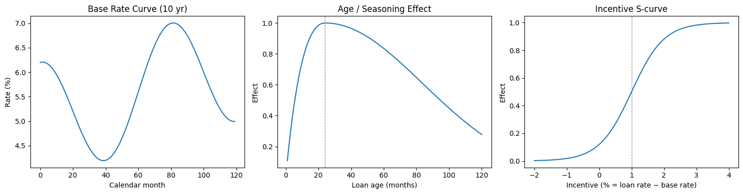
We set up a synthetic data generation process to simulate mortgage prepayment. The simulation assumes a base rate curve over a 10-year horizon, with 100 loans originated each month. Each loan's monthly prepayment probability is driven by three components:

Age seasoning effect $f_{\text{age}}(a)$ : a ramp that starts at 0, peaks around month 24, then slowly decays.
Rate incentive effect $f_{\text{incentive}}(r)$ : an S-curve in the difference between the loan's coupon rate and the prevailing market rate. When the incentive is large (i.e., the borrower can refinance at a much lower rate), prepayment probability climbs sharply.
Interaction: an $f_{\text{age}} \times f_{\text{incentive}}$ cross term, so the two effects are not purely additive.

To make the experiment deliberately challenging for a simple additive GAM, the true data-generating process uses a complementary log-log (cloglog) link with heteroscedastic noise:

\eta_i = \beta_0 + \beta_1 f_{\text{age}}(a_i) + \beta_2 f_{\text{incentive}}(r_i) + \beta_3 f_{\text{age}}(a_i) \cdot f_{\text{incentive}}(r_i) + \varepsilon_i

p_i = 1 - \exp\!\bigl(-\exp(\eta_i)\bigr)

where $\varepsilon_i \sim \mathcal{N}(0,\, \sigma_0 + \sigma_1 f_{\text{incentive}}(r_i))$ . The noise variance grows with the incentive effect, and the cloglog link means the model is asymmetric — it is not a logit.

The actual binary outcome (prepaid or not) is then drawn from a Bernoulli distribution: $y_i \sim \text{Bernoulli}(p_i)$ .

The three component curves (base rate, age effect, incentive S-curve) are shown below:

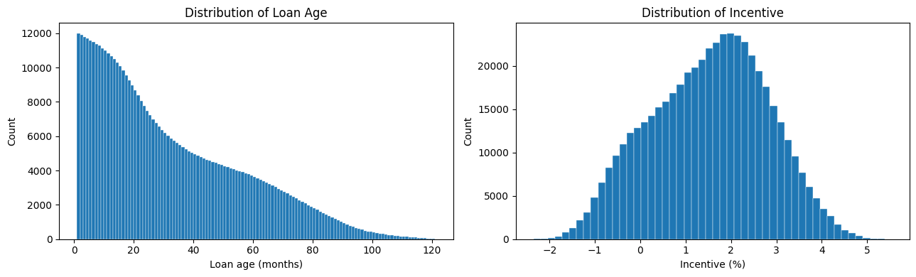
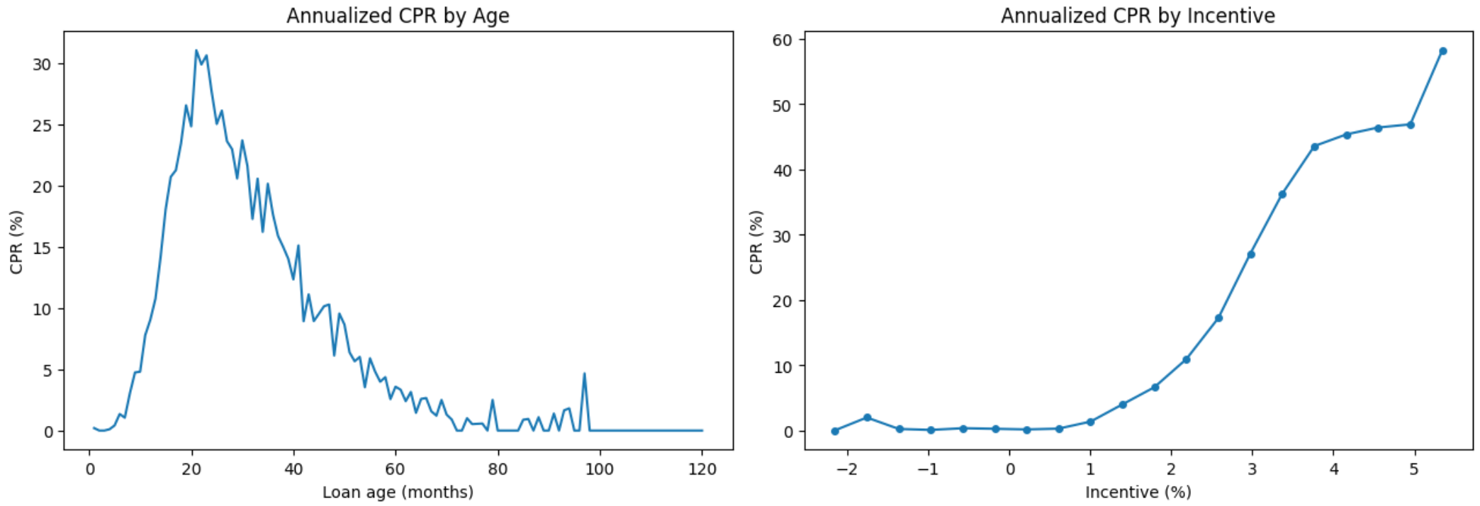
This process generates a panel of roughly 500k loan-month observations, with a true event rate of about 1%. The overall data distribution looks like:

Downsampling

The idea is straightforward: keep all positive events (prepaid = 1), and randomly subsample the non-events until we reach a target event rate.

For instance, we start with 500k observations, of which 5k are positive events (1% event rate). If we target a 10% event rate, we keep all 5k positive events and randomly sample 45k from the 495k non-events, yielding a 50k-row dataset.

The King–Zeng Intercept Correction

Since we have artificially inflated the event rate, a model fitted on the downsampled data will produce predicted probabilities that are biased upward. We need a correction to shift them back to the correct scale.

A well-known fix comes from King and Zeng (2001). Their key insight is that for a logistic model, downsampling the majority class is equivalent to shifting the intercept. We can therefore fit the model on the downsampled data and correct the predictions afterward by shifting them on the log-odds (logit) scale.

Even though the true DGP uses a cloglog link, we fit a standard GAM with a binomial family (logit link) — a deliberate mismatch. The fitted model has the form:

\text{logit}(p_i) = \beta_0 + f_{\text{age}}(a_i) + f_{\text{incentive}}(r_i)

Let $\pi_{\text{true}}$ be the event rate in the full data and $\pi_{\text{down}}$ be the event rate in the downsampled data. The King–Zeng correction term is:

\Delta = \log\!\left(\frac{\pi_{\text{true}}\,(1 - \pi_{\text{down}})}{\pi_{\text{down}}\,(1 - \pi_{\text{true}})}\right)

The corrected predicted probability is then:

\hat{p}_{\text{corrected}} = \sigma\!\bigl(\text{logit}(\hat{p}) + \Delta\bigr)

where $\sigma(x) = \frac{1}{1 + e^{-x}}$ is the sigmoid function, the inverse of the logit.

In our case, $\Delta$ is negative because $\pi_{\text{true}} < \pi_{\text{down}}$ . Intuitively, the model's raw predictions live on the logit scale — the x-axis of the sigmoid function. Adding a negative $\Delta$ shifts those logit values to the left. After applying the sigmoid to map back to probabilities, the leftward-shifted values land on a lower part of the curve:

Sigmoid correction diagram

Applying the Correction: `offset` vs. Post-hoc

There are two ways to apply the King–Zeng correction in practice.

Option 1: offset() during fitting. In mgcv (bam documentation), an offset() term is added directly to the linear predictor. We include $-\Delta$ as the offset so that the model fits the downsampled data while its predictions are already on the original scale. At prediction time on the full data, we set the offset to 0, and the predictions come out correctly with no further adjustment:

\text{logit}(\hat{p}) = \beta_0 + f_{\text{age}}(a_i) + f_{\text{incentive}}(r_i) + \text{offset}

where offset $= -\Delta$ during fitting and offset $= 0$ at prediction time.

Option 2: Post-hoc correction. Alternatively, fit the model on the downsampled data without any offset. Then at prediction time, manually shift the predicted log-odds by $\Delta$ and apply the sigmoid:

\hat{p}_{\text{corrected}} = \sigma\!\bigl(\text{logit}(\hat{p}) + \Delta\bigr)

This approach is more flexible — it does not require baking the correction into the model object.

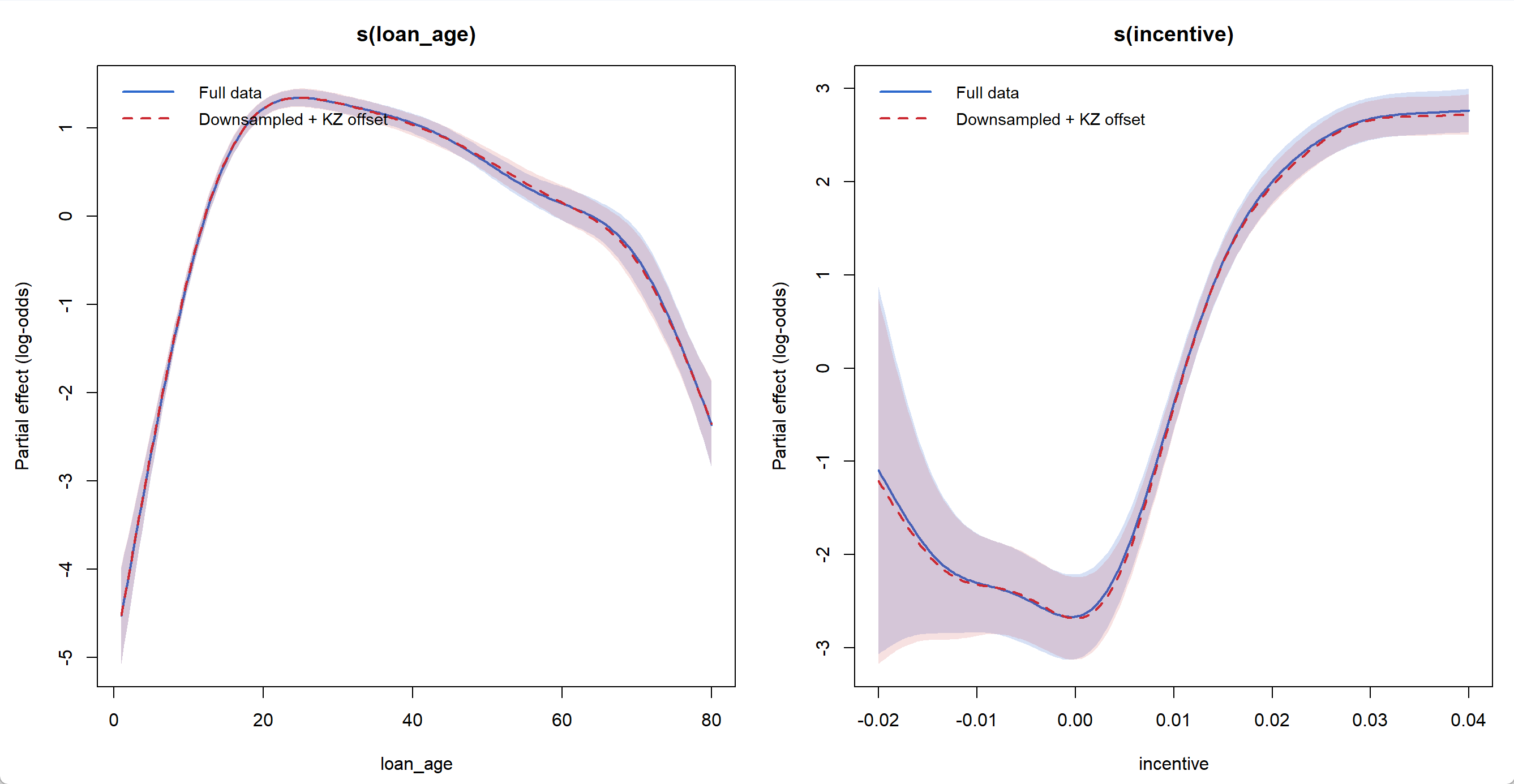
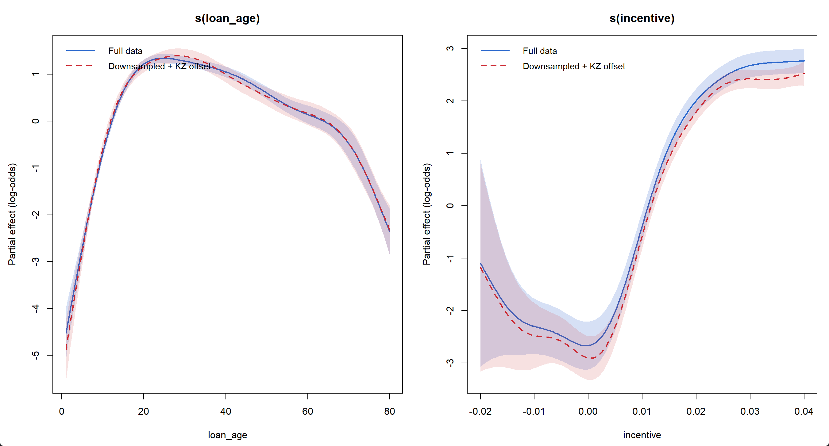
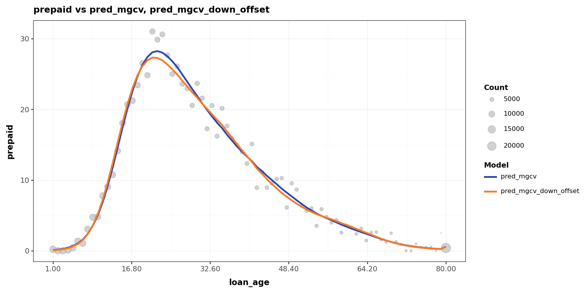
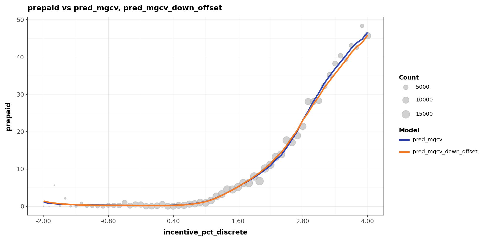
Smooth Curves: Full Data vs. Downsampled + Correction

In my experiments, raising the event rate from 1% to 10% preserves the smooth curve shapes well, and in-sample fitting performance stays almost the same.

From 1% to 10% event rate

From 1% to 50% event rate

When I pushed the target event rate to 50%, the smooth curves started to diverge noticeably — particularly the incentive curve, which becomes more wiggly at both tails where data is sparse.

The reason is that in data-sparse regions, aggressive downsampling amplifies the relative weight of positive events. What was originally noise gets treated by the model as a real pattern, since all positive events are retained while most non-events are discarded. This curve distortion also affects in-sample fitting performance:

Y-axis shows CPR level

More Wiggly or More Flat?

Depending on the local data density, downsampling can distort smooth curves in either direction:

More wiggly curves: in sparse regions, a few positive events that are essentially noise become disproportionately influential after downsampling. The model fits to them as if they were a real pattern, inflating the local event rate and producing spurious curvature.

More flat curves: in dense regions where the true event rate is low but the pattern is genuine and well-supported by volume, downsampling can strip away much of the supporting data. With fewer observations, the smoothing penalty dominates and the model flattens the curve, losing a real signal.

What Else to Consider?

In my other experiments, I have observed that the curve discrepancy from downsampling tends to be larger when:

The features have interactions or there are omitted features the model doesn't capture.
The true link function differs from logit. In practice, the further the real data deviates from a logistic model, the less cleanly a global offset can fix the bias.